In 2005, I developed the
2D gel correlation technique because it was
the only viable method to analyze the data we received at that time.
The company I worked for tried to patent this method
(which was a silly thing to do anyway, its software) and
received feedback from the UK patent office that the method was
already 'invented' in 1975. Of course, since the 70's improvements
in computer processing power makes that the method can now produce
larger volume results. If you are interested in a demonstration
dataset then please have a look
here
Overview
The method correlates the content of multiple 2D gels
with some external parameter (survival rate for instance) and will
report the correlation using a hue color scheme. There is a
 movie
available that summarizes the following steps.
In the examples below, nothing of the biological
information is correct. The examples give an overview of how the
method work and don't make any biological sense. Even the reference to
the 'age' parameter is wrong.
movie
available that summarizes the following steps.
In the examples below, nothing of the biological
information is correct. The examples give an overview of how the
method work and don't make any biological sense. Even the reference to
the 'age' parameter is wrong.
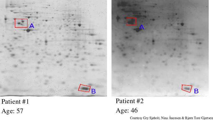
First one starts with a large collection of 2D gels (for instance of
AML/ALL patients). Each of these gels is associated with an extra
parameter, such as survival rate, age, disease type and so on. The
question one now asks is whether there is a relation between spots on
the 2D gels and that specific parameter. E.g: does specific spots
correlate towards the age ?
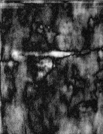
Step 1: Align all images
The first step in the process concerns itself with aligning all the
images such that each pixel on each aligned image reflects the same pI
(horizontally) and protein mass (vertically). This step might require
rotation, zooming and translation of each individual image. Important
here is to realize that cumulative superposition schemes do not work
properly. The image above shows the superposition of 128 aligned
images.
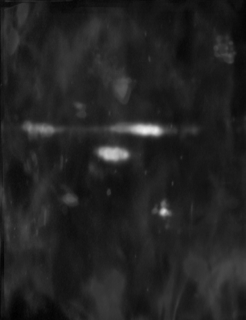
Step 2: Normalize all images
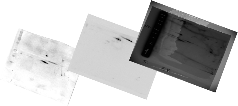
Once the images are aligned, we need to make sure that we can compare
the data between the different images. Often this might require
contrast and brightness alterations. E.g: In the images above we clearly see
that the background is different on the three images. Normalization
will remove these differences.
Step 3: Correlate
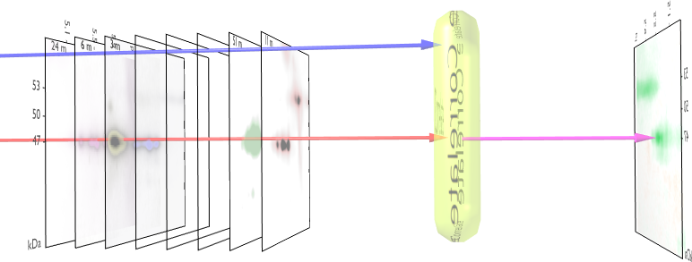
The correlation image can then be computed using for instance the
Spearman Rank order correlation. This is done on an individual pixel
basis and leads to images such as the following:
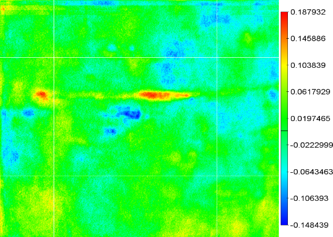
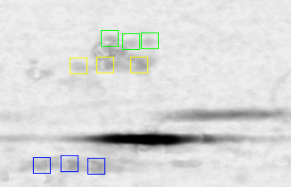
Step 4: Masking
The problem with the above image is that it shows some useless
information. Areas on the gel where we have a correlation but where
the gel content does not alter sufficiently are not useful. Neither
are areas where the probability that that specific correlation might
occur by chance. To mask these areas we create two new images. One for
the variability on the gel and one for the correlation significance.
See figures below:
 |
 |
| The significance mask |
The variance mask |
When these two masks are combined into the correlation image we get
the much more understandable correlation map:
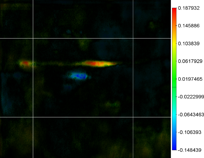
In this image, the areas where the image is red reflect the areas on
the gels where we will tend to find protein for elderly patients.
Where the image is blue we will find that older patients have less
protein expression.
Step 5: Creating the 3D volumetric map
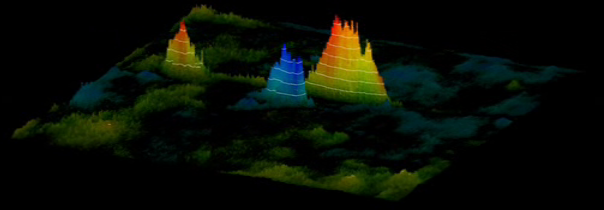
To have a better understanding of which spots correlate with the
external parameter it is useful to map this 2D gel in 3 dimensions.
The 3th dimension is then used to reflect the correlation
strength. Such volumetric maps can even be rotated:
Rotating the 3D volumetric view of the 2D correlation map
Ordering
If you are interested in this analysis feel free to contact werner@yellowcouch.org with
the following tentative information: checklist
- http://analysis.yellowcouch.org/